noreden provides user-friendly functions to facilitate
sustainable diet discovery. Given information for food (groups) and
their nutritional and environmental impact information, the aim is to
find a new diet (i.e. set of foods) that is healthy, acceptable, yet
more sustainable in terms of environmenal impact.
The optimization problem implemented minimizes the difference between the current and new target diet, subject to a set of inequality constraints with respect to nutrition and environmental impact. More details can be found in this document: Optimization (replace link)
In order to find a new diet, you need the following input data:
- current diet: food group names and intake (gram) for each food group
- nutrition (per unit): used to compute total nutrition, such as energy, protein.
- environment impact (per unit): used to compute total impact, such as ghge (green house gas emission)
- constraint: we implement two inequality constraints for each nutrition / env impact, such that the total amount (‘contribution’) falls within a range. In this package the values are based on current diet’s total contribution.
An example
We use a simple example to demonstrate the main features of the package. To get started, load the package.
Process input
We need some information on the current diet we wish to optimize. For now, we use the average diet summarized from a Norwegian dietary survey. However in the future we shall implement flexible input options so that you can insert it yourself.
head(all_diet)
#> # A tibble: 6 × 4
#>   food_name    intake_mean intake_lwr intake_upr
#>   <chr>              <dbl>      <dbl>      <dbl>
#> 1 Bread             188.       18.8        344.
#> 2 Other grains       48.3       4.83       156.
#> 3 Cakes              38.2       3.82       142.
#> 4 Potatoes           72.8       7.28       231.
#> 5 Vegetables        166.       16.6        420.
#> 6 Legumes             3.76      0.376       30.7
We also need the contribution per unit (refered to as
cpu) for each of the food. The food unit is per gram, and
units for nutrition and environmental impact depends on the outcome.
head(contrib_per_unit)
#> # A tibble: 6 × 10
#>   food_name    energy protein  carbs   sugar  fiber     fat vitaminc calcium
#>   <chr>         <dbl>   <dbl>  <dbl>   <dbl>  <dbl>   <dbl>    <dbl>   <dbl>
#> 1 Bread         10.7   0.0912 0.441  0.00285 0.0633 0.0302   0.00570  0.336
#> 2 Other grains  14.0   0.1    0.607  0.0133  0.0578 0.0422   0        0.4
#> 3 Cakes         14.2   0.0674 0.424  0.185   0.0225 0.152    0        0.590
#> 4 Potatoes       3.79  0.0206 0.178  0       0.0177 0.00737  0.133    0.0885
#> 5 Vegetables     1.57  0.0149 0.0498 0.00517 0.0207 0.00841  0.207    0.259
#> 6 Legumes        8.57  0.143  0.286  0       0.0857 0.0286   0        0.571
#> # ℹ 1 more variable: ghge <dbl>
Select food and outcomes of interest
We select 12 foods, and 5 outcomes of interest.
tag_food_12 <- c('Bread', 'Vegetables', 'Red meat',
                'Milk, yoghurt', 'Fish', 'Cheese',
                'Eggs', 'Fruit, berries', 'Potatoes',
                'Other grains', 'Butter, margarine, oil', 'Sugar, sweets')

tag_outcome_5 <- c('energy', 'protein', 'carbs', 'fat', 'ghge')
For the current diet selection, we get the average diet
(intake_mean) as a baseline, from which we search for a new
diet that satisfy our requirements; in addition, we also get the upper
and lower bound for the new diet so that it is not too far from the
current one.
diet_selected <- select_diet(
  data_diet = all_diet,
  tag_food = tag_food_12)

diet_selected
#> # A tibble: 12 × 4
#>    food_name              intake_mean intake_lwr intake_upr
#>    <chr>                        <dbl>      <dbl>      <dbl>
#>  1 Bread                        188.       18.8       344.
#>  2 Other grains                  48.3       4.83      156.
#>  3 Potatoes                      72.8       7.28      231.
#>  4 Vegetables                   166.       16.6       420.
#>  5 Fruit, berries               184.       18.4       553.
#>  6 Red meat                     126.       12.6       300.
#>  7 Fish                          74.6       7.46      303.
#>  8 Eggs                          26.4       2.64      112.
#>  9 Milk, yoghurt                329.       32.9       901.
#> 10 Cheese                        46.6       4.66      122.
#> 11 Butter, margarine, oil        32.3       3.23       71.4
#> 12 Sugar, sweets                 18.1       1.81       66
Do the same for outcomes on selected foods.
cpu_selected <- select_perunit(
  data_perunit_contrib = contrib_per_unit,
  tag_food = tag_food_12,
  tag_outcome = tag_outcome_5)
cpu_selected
#> # A tibble: 12 × 6
#>    food_name              energy protein   carbs     fat    ghge
#>    <chr>                   <dbl>   <dbl>   <dbl>   <dbl>   <dbl>
#>  1 Bread                   10.7  0.0912  0.441   0.0302  0.00107
#>  2 Other grains            14.0  0.1     0.607   0.0422  0.00235
#>  3 Potatoes                 3.79 0.0206  0.178   0.00737 0.00037
#>  4 Vegetables               1.57 0.0149  0.0498  0.00841 0.00103
#>  5 Fruit, berries           2.73 0.00758 0.134   0.00408 0.00072
#>  6 Red meat                 8.34 0.173   0.0136  0.139   0.0129
#>  7 Fish                     6.09 0.170   0.0245  0.0748  0.00311
#>  8 Eggs                     6.18 0.130   0.00407 0.106   0.00215
#>  9 Milk, yoghurt            1.98 0.0359  0.0559  0.0111  0.00143
#> 10 Cheese                  13.5  0.217   0.0484  0.242   0.0103
#> 11 Butter, margarine, oil  23.4  0.0133  0.0233  0.615   0.00467
#> 12 Sugar, sweets           18.0  0.0533  0.609   0.178   0.00387
Compute total contribution
We compute the total contribution of the food combination. This is the basis when we search for new diet that satisfies the nutrition and environmental constraints.
tc <- compute_total_contrib(
  data_diet = diet_selected,
  data_perunit_contrib = cpu_selected)

tc
#> $total_contrib
#>   tag_outcome total_contrib
#> 1      energy   7762.508053
#> 2     protein     88.576337
#> 3       carbs    194.438480
#> 4         fat     74.404123
#> 5        ghge      3.739236
#>
#> $tag_food
#>  [1] "Bread"                  "Other grains"           "Potatoes"
#>  [4] "Vegetables"             "Fruit, berries"         "Red meat"
#>  [7] "Fish"                   "Eggs"                   "Milk, yoghurt"
#> [10] "Cheese"                 "Butter, margarine, oil" "Sugar, sweets"
#>
#> $tag_outcome
#> [1] "energy"  "protein" "carbs"   "fat"     "ghge"
Set constraints
The inequality constraints look like this:
- total energy <= upper bound for energy
- total energy >= lower bound for energy
By default we can set the upper bound to be the same as the current total outputs, and lower bound to be 90% of the current total outputs.
constr_coef_df <- set_constr_coef(
  tag_outcome = tag_outcome_5,
  coef_lwr = rep(0.9, length(tag_outcome_5)),
  coef_upr = rep(1.0, length(tag_outcome_5)))
constr_coef_df
#>   tag_outcome coef_constrlwr coef_construpr
#> 1      energy            0.9              1
#> 2     protein            0.9              1
#> 3       carbs            0.9              1
#> 4         fat            0.9              1
#> 5        ghge            0.9              1
When we try to reduce the output in a specific outcome (such as
ghge), we can set it to be 90% the previous level: the function
reduce_constr() allows you to set it.
# reduce ghge to 0.9
constr_coef_df_red <- reduce_constr(
  data_constr_coef = constr_coef_df,
  tag_outcome_reduce = 'ghge',
  coef_reduce = 0.9)
constr_coef_df_red
#>   tag_outcome coef_constrlwr coef_construpr
#> 1      energy           0.90            1.0
#> 2     protein           0.90            1.0
#> 3       carbs           0.90            1.0
#> 4         fat           0.90            1.0
#> 5        ghge           0.81            0.9
Use total contribution and constraint coefficients to compute the upper and lower bound.
constr_val_reduce <- compute_constr(
  data_total_contrib = tc$total_contrib,
  data_constr_coef = constr_coef_df_red)
constr_val_reduce
#>   tag_outcome total_contrib coef_constrlwr coef_construpr  constr_lwr
#> 1      energy   7762.508053           0.90            1.0 6986.257248
#> 2     protein     88.576337           0.90            1.0   79.718703
#> 3       carbs    194.438480           0.90            1.0  174.994632
#> 4         fat     74.404123           0.90            1.0   66.963711
#> 5        ghge      3.739236           0.81            0.9    3.028781
#>    constr_upr
#> 1 7762.508053
#> 2   88.576337
#> 3  194.438480
#> 4   74.404123
#> 5    3.365312
Set standardized constraints
Sometimes it is better for computaion to use standardized values rather than the original. We have implemented one way to standardize.
stdcoef <- compute_stdcoef(data_perunit_contrib = cpu_selected)
stdcoef
#> $std_coef
#>   tag_outcome    std_coef
#> 1      energy   0.1449335
#> 2     protein  13.7615608
#> 3       carbs   4.3037780
#> 4         fat   5.7738141
#> 5        ghge 251.6962095
#>
#> $method
#> [1] "sd"

cpu_selected_std_res <- compute_std_unit_contrib(
  uc_raw = cpu_selected,
  std_coef = stdcoef$std_coef)

cpu_selected_std <- cpu_selected_std_res$uc_std

# total contrib (std)
tc_std <- compute_total_contrib(
  data_diet = diet_selected,
  data_perunit_contrib = cpu_selected_std)
tc_std
#> $total_contrib
#>   tag_outcome total_contrib
#> 1      energy     1125.0477
#> 2     protein     1218.9486
#> 3       carbs      836.8200
#> 4         fat      429.5956
#> 5        ghge      941.1514
#>
#> $tag_food
#>  [1] "Bread"                  "Other grains"           "Potatoes"
#>  [4] "Vegetables"             "Fruit, berries"         "Red meat"
#>  [7] "Fish"                   "Eggs"                   "Milk, yoghurt"
#> [10] "Cheese"                 "Butter, margarine, oil" "Sugar, sweets"
#>
#> $tag_outcome
#> [1] "energy"  "protein" "carbs"   "fat"     "ghge"
Now we directly use the 90% ghge constraint coefficients.
# constraints based on std total contrib
constr_val_reduce_std <- compute_constr(
  data_total_contrib = tc_std$total_contrib,
  data_constr_coef = constr_coef_df_red)

constr_val_reduce_std
#>   tag_outcome total_contrib coef_constrlwr coef_construpr constr_lwr constr_upr
#> 1      energy     1125.0477           0.90            1.0  1012.5430  1125.0477
#> 2     protein     1218.9486           0.90            1.0  1097.0538  1218.9486
#> 3       carbs      836.8200           0.90            1.0   753.1380   836.8200
#> 4         fat      429.5956           0.90            1.0   386.6360   429.5956
#> 5        ghge      941.1514           0.81            0.9   762.3326   847.0363
Find new diet
In order to run the algorithm to search for new diet, we need to provide the algorithm the data we prepared from previous steps in a format that is ordered by outcome.
Here we use the standardized constraints for numerical stability.
# split constraint values
constval <- values_by_tag_outcome(
  data_unit_contrib = cpu_selected_std,
  data_constr = constr_val_reduce_std)

constval$food_name
#>  [1] "Bread"                  "Other grains"           "Potatoes"
#>  [4] "Vegetables"             "Fruit, berries"         "Red meat"
#>  [7] "Fish"                   "Eggs"                   "Milk, yoghurt"
#> [10] "Cheese"                 "Butter, margarine, oil" "Sugar, sweets"
constval$tag_outcome
#> [1] "energy"  "protein" "carbs"   "fat"     "ghge"

# for energy, unit_contrib per food, lwr and upr bound of total contrib
constval$val$energy
#> $unit_contrib
#>  [1] 1.5501443 2.0322902 0.5493793 0.2268688 0.3955038 1.2090119 0.8821135
#>  [8] 0.8955243 0.2869315 1.9569367 3.3898076 2.6070884
#>
#> $lwr
#> [1] 1012.543
#>
#> $upr
#> [1] 1125.048
Run the optimization, and retrieve the new diet along with current diet.
res <- find_new_diet(diet0 = diet_selected$intake_mean,
                     diet0_upr = diet_selected$intake_upr,
                     diet0_lwr = diet_selected$intake_lwr,
                     tag_outcomes = tag_outcome_5,
                     constraint_val = constval$val,
                     print_runtime = T)
# collect result
new_diet <- return_new_diet(
  result_obj = res$run_optim,
  data_current_diet = diet_selected)
new_diet
#>                 food_name       new   current
#> 1                   Bread 187.11762 188.31866
#> 2            Other grains  45.56513  48.31437
#> 3                Potatoes  72.37999  72.79364
#> 4              Vegetables 164.71925 165.98669
#> 5          Fruit, berries 183.25414 184.13142
#> 6                Red meat 110.39761 126.26154
#> 7                    Fish  71.10191  74.61885
#> 8                    Eggs  24.33138  26.41185
#> 9           Milk, yoghurt 326.87133 328.64505
#> 10                 Cheese  35.17652  46.59652
#> 11 Butter, margarine, oil  30.50184  32.31694
#> 12          Sugar, sweets  14.33111  18.14473
Present the results
We can show some useful comparisons between the two diets, in terms of absolute and relative percent change.
# compute difference
new_old_compare <- compare_new_diet(data_new_diet = new_diet,
                 data_current_diet = diet_selected)

new_old_compare
#>                 food_name    new current current_lwr current_upr abs_change
#> 1                   Bread 187.12  188.32       18.83       343.8      -1.20
#> 2            Other grains  45.57   48.31        4.83       155.7      -2.75
#> 3                Potatoes  72.38   72.79        7.28       230.7      -0.41
#> 4              Vegetables 164.72  165.99       16.60       419.7      -1.27
#> 5          Fruit, berries 183.25  184.13       18.41       552.7      -0.88
#> 6                Red meat 110.40  126.26       12.63       299.6     -15.86
#> 7                    Fish  71.10   74.62        7.46       302.9      -3.52
#> 8                    Eggs  24.33   26.41        2.64       111.6      -2.08
#> 9           Milk, yoghurt 326.87  328.65       32.86       900.6      -1.77
#> 10                 Cheese  35.18   46.60        4.66       121.6     -11.42
#> 11 Butter, margarine, oil  30.50   32.32        3.23        71.4      -1.82
#> 12          Sugar, sweets  14.33   18.14        1.81        66.0      -3.81
#>    perc_change
#> 1        -0.01
#> 2        -0.06
#> 3        -0.01
#> 4        -0.01
#> 5         0.00
#> 6        -0.13
#> 7        -0.05
#> 8        -0.08
#> 9        -0.01
#> 10       -0.25
#> 11       -0.06
#> 12       -0.21
We can also validate whether the new diet satisfies the constraints.
# validate constraints
new_diet_validate <- validate_diet_contrib(data_new_diet = new_diet,
                      data_unit_contrib = cpu_selected,
                      data_constr = constr_val_reduce)

new_diet_validate
#>   tag_outcome total_contrib_new total_contrib coef_constrlwr coef_construpr
#> 1      energy           7269.81       7762.51           0.90            1.0
#> 2     protein             81.79         88.58           0.90            1.0
#> 3       carbs            188.66        194.44           0.90            1.0
#> 4         fat             66.96         74.40           0.90            1.0
#> 5        ghge              3.37          3.74           0.81            0.9
#>   constr_lwr constr_upr check deviation
#> 1    6986.26    7762.51    ok         0
#> 2      79.72      88.58    ok         0
#> 3     174.99     194.44    ok         0
#> 4      66.96      74.40    ok         0
#> 5       3.03       3.37    ok         0
It is possible to visualize the results or present results in better looking tables.
d_compare_gram <- prep_diet_comparison_gram(
  new_old_compare)

p1 <- plot_diet_comparison_gram(plot_obj = d_compare_gram,
                          title_text = 'New diet',
                          axis_x_text = 'Food groups',
                          axis_y_text = 'Intake (grams)')

d_compare_percent <- prep_diet_comparison_percent(
  data_dietsummary = new_old_compare)

p2 <- plot_diet_comparison_percent(plot_obj = d_compare_percent,
                                   title_text = 'Percent change',
                                   axis_x_text = 'Food groups',
                                   axis_y_text = 'Percent')

library(patchwork)
p1 + p2 + plot_layout(nrow = 1)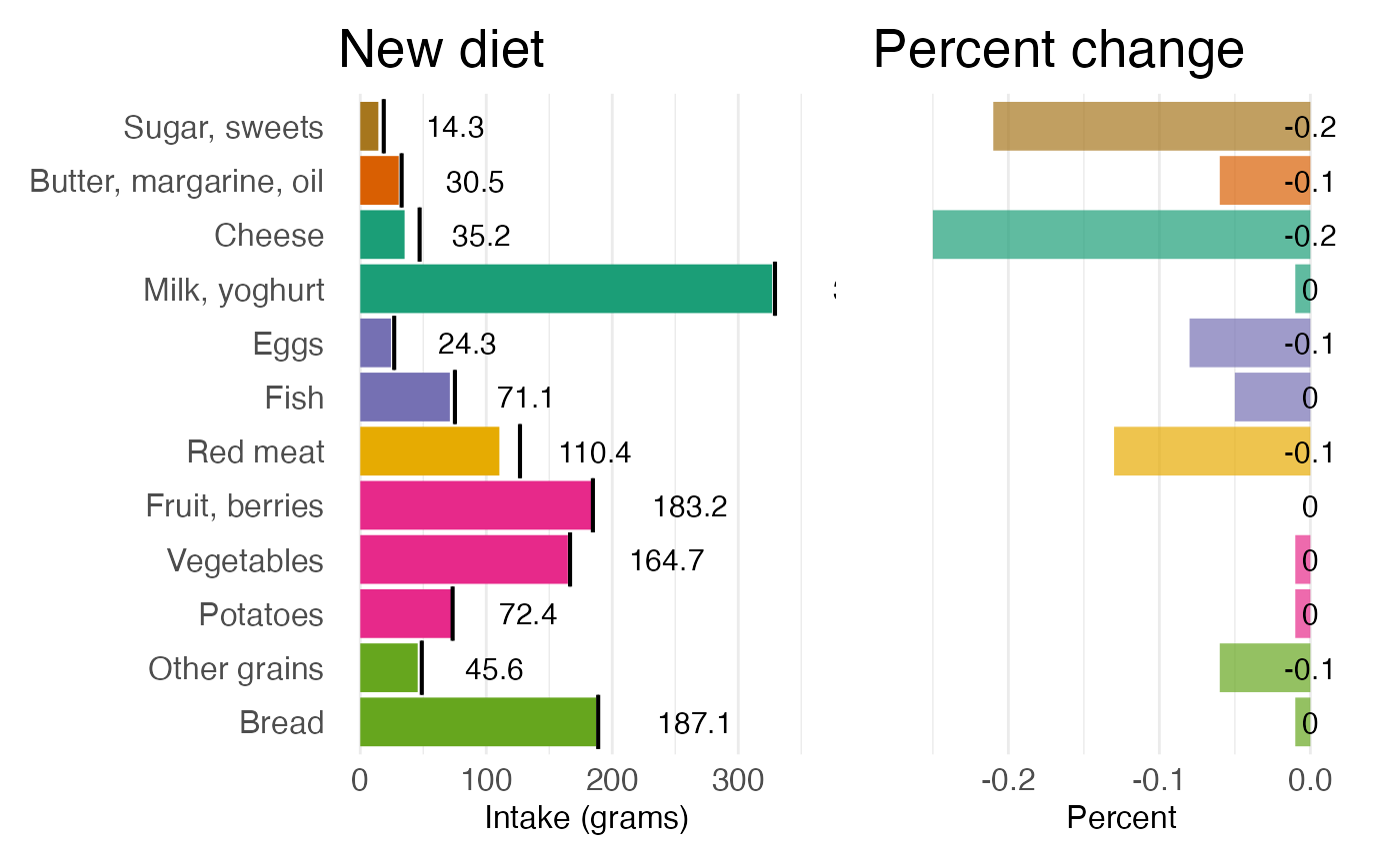
Table with comments.
d_tb_validate <- prep_validate_table(
  data_validate_diet = new_diet_validate)
table_validate(d_tb_validate)| Outcome | Total contribution | Constraint | ||
|---|---|---|---|---|
| New diet | Current diet | Range | Comments | |
| energy | 7269.81 | 7762.51 | 6986.26‐7762.51 | Ok |
| protein | 81.79 | 88.58 | 79.72‐88.58 | Ok |
| carbs | 188.66 | 194.44 | 174.99‐194.44 | Ok |
| fat | 66.96 | 74.40 | 66.96‐74.40 | Ok |
| ghge | 3.37 | 3.74 | 3.03‐3.37 | Ok |